
DX-COM Configuration Reference
A complete parameter reference for DX-COM's config.json covering input shapes, calibration settings, PPU post-processing for YOLO models, DXQ accuracy recovery, and every preprocessing operation, with copy-ready examples.
DX-COM Configuration Reference
Every parameter in config.json, the file that drives DX-COM, the DEEPX NPU
compiler. Built as a lookup, not a walkthrough: jump to the field you need, copy a
validated example, ship.
config.json file?
config.json is the single file that controls how DX-COM interprets your model.
It has six top-level keys: four required (inputs,
calibration_method, calibration_num, default_loader)
and two optional (enhanced_scheme for DXQ accuracy recovery, ppu
for hardware-accelerated detection post-processing).
Top-level structure
A complete configuration has six top-level keys: four required, two optional. Click a card below to jump straight to its parameter reference.
Model input tensor name and shape [batch, channels, height, width].
Algorithm used to estimate INT8 quantisation ranges.
Number of calibration samples to process. Trades compile time for accuracy.
Calibration dataset path, accepted file types, and the preprocessing pipeline.
DXQ accuracy-recovery schemes. Use when INT8 accuracy drops too far from FP32.
Post-Processing Unit for object detection. Offloads filtering and class selection to the NPU.
A minimal skeleton with every top-level key in place:
{
  "inputs":             { ... },
  "calibration_method": "...",
  "calibration_num":    100,
  "default_loader":     { ... },
  "enhanced_scheme":    { ... },  // optional
  "ppu":                { ... }   // optional
}
inputs
Defines the input tensor name and shape of your ONNX model.
inputs
{
  "inputs": {
    "images": [1, 3, 640, 640]
  }
}
The key ("images") must exactly match the input tensor name in your ONNX
graph. The value is the shape array [batch, channels, height, width].
| Dimension | Position | Notes |
|---|---|---|
| Batch size | [0] | Must be 1. DX-COM does not support dynamic or multi-batch compilation via the CLI. |
| Channels | [1] | 3 for RGB or BGR images, 1 for grayscale |
| Height | [2] | Input image height in pixels |
| Width | [3] | Input image width in pixels |
.onnx file in
Netron, click the first
node in the graph, and read the input name from the left panel. Names are
case-sensitive, copy exactly as shown.
dxcom CLI supports only
single-input models. For multi-input models, use the dx_com Python module
with a custom torch DataLoader.
Calibration parameters
Two parameters control how DX-COM estimates the FP32 → INT8 quantisation ranges.
calibration_method picks the algorithm; calibration_num sets how
many samples it processes.
calibration_method
Specifies the algorithm used to determine quantisation ranges during calibration. Affects how accurately the compiler maps FP32 activation values to INT8 representations.
{
  "calibration_method": "ema"
}
| Value | Algorithm | When to use |
|---|---|---|
"ema" | Exponential Moving Average, smooths activation range estimates across calibration steps | Default choice. Produces better post-quantisation accuracy in most models. |
"minmax" | Absolute minimum and maximum of observed activation values | Useful when activations have predictable, stable ranges with no outliers. |
Start with "ema". Switch to "minmax" only if you have a
specific reason based on your model's activation distribution.
calibration_num
Sets the number of calibration samples the compiler processes to estimate activation ranges. Higher values give the compiler more data to build accurate activation statistics, which can improve quantised accuracy, and increase compilation time proportionally.
{
  "calibration_num": 100
}
| Value | Compile speed | Use case |
|---|---|---|
1 | Very fast | Quick sanity check, verify the pipeline runs end-to-end |
5–10 | Fast | Rapid iteration while tuning your config |
100 | Moderate | Good default for most models |
500–1000 | Slow | When accuracy after quantisation is below your target |
Start with 100. If accuracy drops significantly compared to the original
FP32 model, increase to 500 or 1000. The optimal value depends
on your model and dataset; there is no universal correct answer.
default_loader
Configures the calibration data pipeline: where to find images, which file types to accept, and how to preprocess them before feeding them to the compiler.
default_loader
{
  "default_loader": {
    "dataset_path":    "./calibration_images",
    "file_extensions": ["jpeg", "jpg", "png", "JPEG"],
    "preprocessings": [
      {"resize":       {"width": 640, "height": 640}},
      {"convertColor": {"form": "BGR2RGB"}},
      {"div":          {"x": 255}},
      {"normalize":    {"mean": [0.485, 0.456, 0.406], "std": [0.229, 0.224, 0.225]}},
      {"transpose":    {"axis": [2, 0, 1]}},
      {"expandDim":    {"axis": 0}}
    ]
  }
}
| Field | Type | Description |
|---|---|---|
dataset_path |
string | Path to the directory containing your calibration images. Relative or absolute. The directory should hold representative samples from your deployment domain, calibration quality directly affects quantised accuracy. |
file_extensions |
array<string> | File extensions the loader will accept. Files with other extensions are ignored. Include both lowercase and uppercase variants if your dataset has mixed naming. |
preprocessings |
array<object> | Ordered list of preprocessing operations applied to each calibration image. Operations execute in the order they are listed. See Preprocessing operations. |
The preprocessing pipeline must exactly replicate the preprocessing your model expects at inference time. A mismatch between calibration preprocessing and runtime preprocessing is one of the most common causes of accuracy degradation after quantisation.
The mean and std values above ([0.485, 0.456, 0.406] /
[0.229, 0.224, 0.225]) are standard ImageNet constants for classification
models such as ResNet and MobileNet. YOLO models (v8–v12) do not use this
step, omit normalize from your config when compiling YOLO. For
custom models, use the mean and std values from your training pipeline.
default_loader supports
only image data for single-input models. For non-image data or multi-input
configurations, use the dx_com Python module with a custom torch
DataLoader.
enhanced_scheme — DXQ accuracy recovery
Enables DXQ, a set of accuracy-recovery algorithms that reduce the
accuracy loss introduced by INT8 quantisation. Schemes range from P0 (fast,
modest improvement) to P5 (slow, high improvement).
enhanced_scheme
Use DXQ when your quantised model shows a meaningful accuracy drop compared to the original FP32 model and other approaches, more calibration data, better calibration images, have not resolved it. DXQ significantly increases compilation time; only enable it when needed.
{
  "enhanced_scheme": {
    "DXQ-P3": {
      "num_samples": 1024
    }
  }
}
P3 offers a strong balance between accuracy improvement and compilation
time, and is validated across a wide range of models. If compilation time is too
long, step down to P1 or P2. If P3 is
insufficient, try P4 or P5.
ppu — Post-Processing Unit
The Post-Processing Unit (PPU) is a hardware block inside the DX-M1 NPU designed to accelerate object detection post-processing. Enabling PPU offloads parts of the detection pipeline from the host CPU to the NPU, reducing CPU load and end-to-end latency.
Should I enable PPU?
| Model type | PPU recommendation |
|---|---|
| YOLO object detection (any variant) | Enable — meaningful CPU reduction on edge devices |
| Classification (ResNet, MobileNet, etc.) | Do not enable — these models have no detection head |
| Segmentation (DeepLab, U-Net, etc.) | Do not enable — pixel-level mask processing is incompatible |
| Custom detection architectures | Only if the output tensor structure matches YOLO-style heads |
Non-Maximum Suppression is not supported by PPU. It must always run on the host CPU using the filtered model outputs.
Three PPU paths
Pick the path that matches your model's detection head. If you're using YOLOv8 or later, see the Type 1 vs Type 2 decision below.
| Type | Approach | Hardware used | Supported architectures |
|---|---|---|---|
0 | Anchor-based PPU path | NPU hardware | YOLOv3, v4, v5, v7 |
1 | Anchor-free PPU path | NPU hardware | YOLOX, YOLOv8–v12 |
2 | CPU-side TopK optimisation | CPU only | YOLOv8–v12 (DFL-based, fallback) |
Type 0 — anchor-based models (YOLOv3, v4, v5, v7)
Offloads confidence filtering and Argmax class selection for anchor-based detection heads to the NPU hardware.
ppu — type 0
{
  "ppu": {
    "type":        0,
    "conf_thres":  0.25,
    "activation":  "Sigmoid",
    "num_classes": 80,
    "layer": {
      "Conv_245": {"num_anchors": 3},
      "Conv_294": {"num_anchors": 3},
      "Conv_343": {"num_anchors": 3}
    }
  }
}
| Parameter | Type | Description |
|---|---|---|
type | int | Set to 0 for anchor-based models |
conf_thres | float | Confidence threshold. Detections below this value are filtered at compile time. Fixed at compile time, changing it requires recompilation. |
activation | string | Activation applied to outputs. Typically "Sigmoid" for anchor-based YOLO models. |
num_classes | int | Number of detection classes in your model |
layer | object | Maps Conv node names to their anchor count. Each key is a node name from the ONNX graph. |
Finding layer node names
Open your model in Netron. Trace backward from the model outputs and locate the final
Conv layers in the detection head. For anchor-based models, these Conv layers output
feature maps with shape [1, num_anchors × (5 + num_classes), H, W]. There
is typically one Conv per detection scale (small, medium, large objects).
The output channel count confirms the right node. For example, with 3 anchors and 80
classes: 3 × (5 + 80) = 255. Copy the node name exactly from the Node
Properties panel on the right side of Netron.
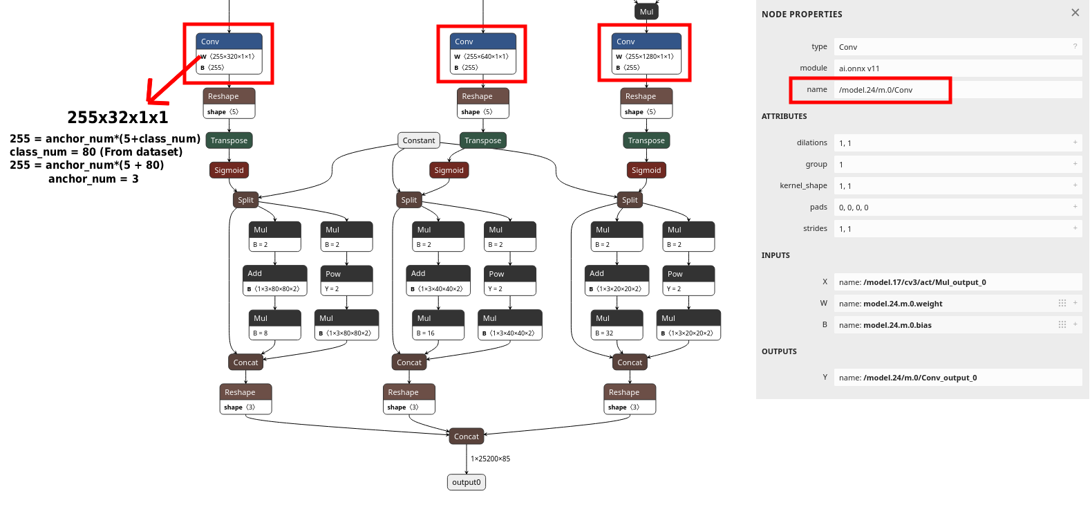
layer config. The Node Properties panel on the right shows the exact name to copy, in this example /model.24/m.0/Conv. The output channel count of 255 confirms the formula: 3 anchors × (5 + 80 classes) = 255.
Type 1 — anchor-free models (YOLOX, YOLOv8–v12)
Offloads confidence filtering and class selection to the NPU hardware for anchor-free
detection architectures. The exact layer structure depends on whether your
model is YOLOX (separate objectness and class confidence branches) or YOLOv8 and later
(merged confidence output).
ppu — type 1 (YOLOX)
{
  "ppu": {
    "type":        1,
    "conf_thres":  0.25,
    "num_classes": 80,
    "layer": [
      {"bbox": "output_bbox_1", "obj_conf": "output_obj_1", "cls_conf": "output_cls_1"},
      {"bbox": "output_bbox_2", "obj_conf": "output_obj_2", "cls_conf": "output_cls_2"},
      {"bbox": "output_bbox_3", "obj_conf": "output_obj_3", "cls_conf": "output_cls_3"}
    ]
  }
}
Finding layer node names
The YOLOX head has three detection scales, each with three separate Conv branches:
bbox, obj_conf, and cls_conf. Locate the Conv node
for each branch at each scale and copy the node names into the layer array,
9 entries total (3 scales × 3 branches). The node name is shown in the Node Properties
panel on the right side of Netron.
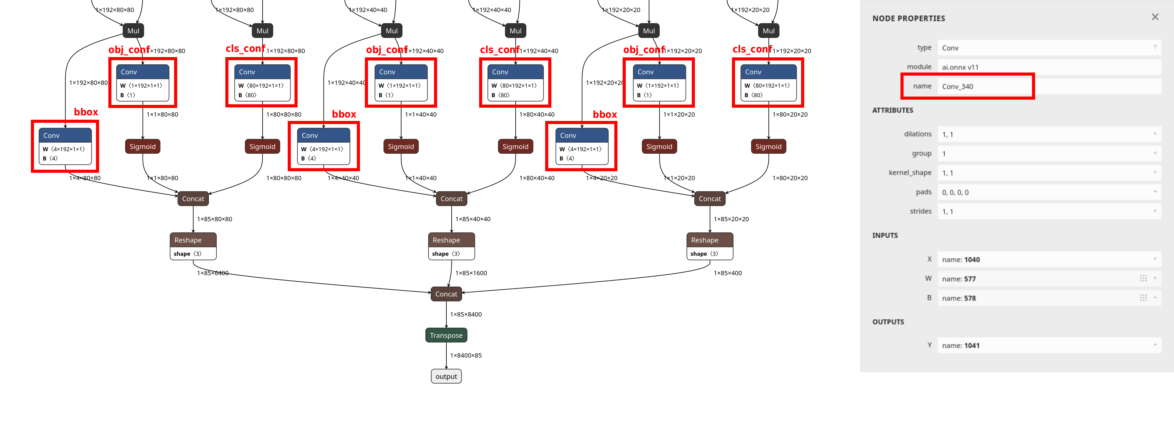
bbox, obj_conf, and cls_conf. The node name is visible in the Node Properties panel on the right, for example Conv_340. These are the values to use in the layer config.
ppu — type 1 (YOLOv8 / v9 / v10 / v11 / v12)
{
  "ppu": {
    "type":        1,
    "conf_thres":  0.25,
    "num_classes": 80,
    "layer": [
      {"bbox": "Mul_441", "cls_conf": "Sigmoid_442"}
    ]
  }
}
Finding layer node names
Open the model in Netron. Locate the final Concat node in the detection
head. Trace backward from it to find the bbox source (the Mul
node) and the cls_conf source (the Sigmoid node). Click each
node to read its exact name from the Node Properties panel on the right.
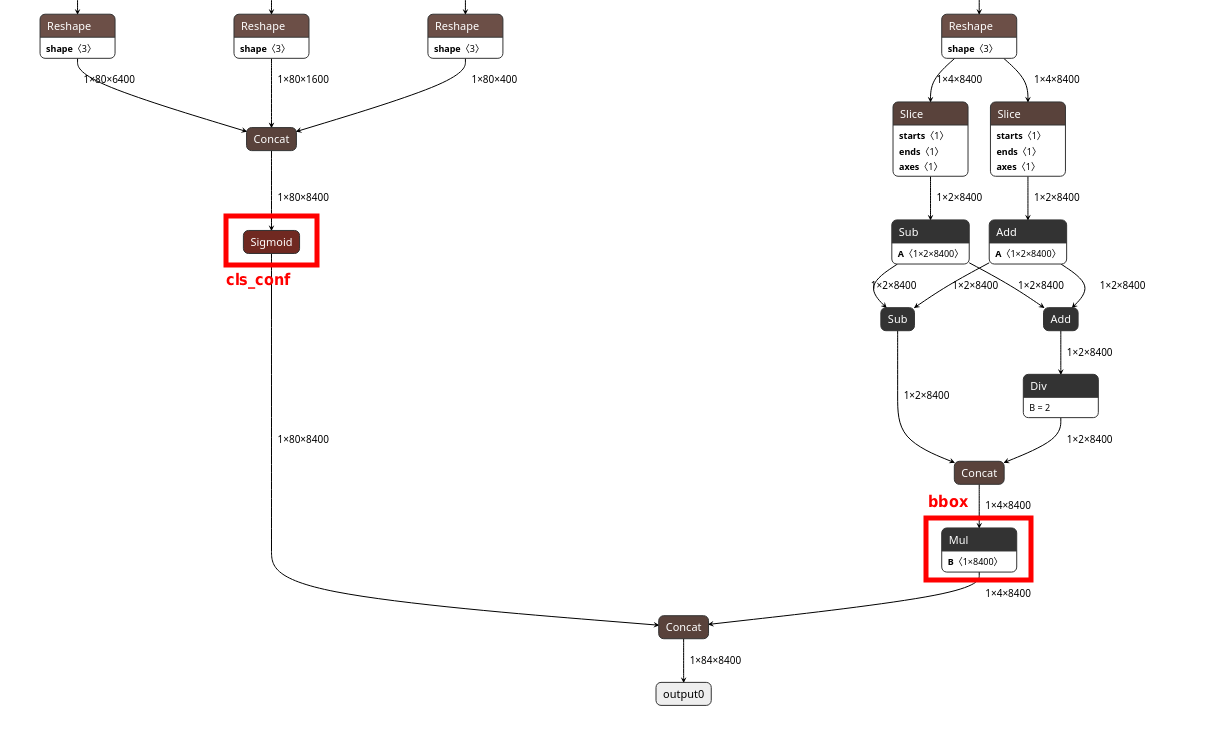
Sigmoid node (left, highlighted in red) is the cls_conf source. The Mul node (right, highlighted in red) is the bbox source. Both nodes feed into the final Concat that produces output0. Click each node to copy its exact name from the Node Properties panel.
Type 1 — parameter reference
| Parameter | Type | Description |
|---|---|---|
type | int | Set to 1 for the standard anchor-free PPU path |
conf_thres | float | Confidence threshold. Fixed at compile time, changing it requires recompilation. |
num_classes | int | Number of detection classes |
layer | array | List of detection head node mappings. Each entry maps tensor roles to ONNX node names. |
Layer entry fields
| Field | YOLOX | YOLOv8–v12 | Description |
|---|---|---|---|
bbox | Required | Required | Bounding box output node name |
obj_conf | Required | Not used | Object confidence node name. YOLOX separates objectness from class confidence; YOLOv8 and later merge them into a single cls_conf output. |
cls_conf | Required | Required | Class confidence node name |
Type 2 — DFL-based anchor-free models, CPU-side TopK (YOLOv8–v12)
type: 2 does not use PPU hardware. It is a CPU-side
optimisation that runs TopK candidate reduction before the DFL decoding and NMS stages.
By reducing the number of candidates that flow into the heavier CPU-side post-processing
steps, it lowers CPU workload and improves runtime efficiency.
Use type: 2 when your model uses a DFL-based head and you can map per-scale
bbox and cls_conf nodes, but the type: 1 mapping is
unavailable or produces a compile error. This path was validated with YOLOv8, v9, v10, v11,
and v12 in DX-COM v2.3.0.
ppu — type 2
{
  "ppu": {
    "type":        2,
    "topk":        512,
    "num_classes": 80,
    "layer": [
      {"bbox": "bbox_head_p3", "cls_conf": "cls_head_p3"},
      {"bbox": "bbox_head_p4", "cls_conf": "cls_head_p4"},
      {"bbox": "bbox_head_p5", "cls_conf": "cls_head_p5"}
    ]
  }
}
| Parameter | Type | Required | Description |
|---|---|---|---|
type | int | Yes | Set to 2 for the CPU-side TopK path |
topk | int | No | Number of candidates kept before DFL decoding. If omitted, DX-COM uses its internal default. 512 is a validated starting point. |
num_classes | int | Yes | Number of detection classes |
layer | array | Yes | Per-scale detection head mappings. Three entries expected, one per detection scale (P3, P4, P5). |
Finding layer node names
Type 2 requires a custom ONNX export where the DFL decoding is removed from the graph,
exposing per-scale bbox and cls_conf Conv nodes directly. Once
exported and simplified, open the model in Netron. For each of the three detection
scales (P3, P4, P5), locate the final bbox Conv node and the final
cls_conf Conv node and copy their names into the layer array.
Type 1 vs Type 2 — which should you use?
For YOLOv8 and later, both paths are valid. Use this matrix to pick the right one.
Type 1 — NPU hardware path
"type": 1
bbox and cls_conf layer names from your ONNX export.
Type 2 — CPU-side TopK
"type": 2
Complete configuration examples
Two end-to-end configurations you can copy into your own project as a starting point. Both have been compiled against DX-COM v2.3.0.
Classification model (no PPU)
A typical ImageNet-style classification model (ResNet, MobileNet, EfficientNet) with standard normalisation and 224×224 input.
{
  "inputs":             {"input": [1, 3, 224, 224]},
  "calibration_method": "ema",
  "calibration_num":    100,
  "default_loader": {
    "dataset_path":    "./calibration_images",
    "file_extensions": ["jpeg", "jpg", "png", "JPEG"],
    "preprocessings": [
      {"resize":       {"width": 224, "height": 224}},
      {"convertColor": {"form": "BGR2RGB"}},
      {"div":          {"x": 255}},
      {"normalize":    {"mean": [0.485, 0.456, 0.406], "std": [0.229, 0.224, 0.225]}},
      {"transpose":    {"axis": [2, 0, 1]}},
      {"expandDim":    {"axis": 0}}
    ]
  }
}
YOLOv11n with PPU type 1
YOLOv11n object detection at 640×640 with hardware-accelerated post-processing. Note the
absence of normalize, YOLO models do not use ImageNet normalisation.
{
  "inputs":             {"images": [1, 3, 640, 640]},
  "calibration_method": "ema",
  "calibration_num":    100,
  "default_loader": {
    "dataset_path":    "./calibration_images",
    "file_extensions": ["jpeg", "jpg", "png", "JPEG"],
    "preprocessings": [
      {"resize":       {"width": 640, "height": 640}},
      {"convertColor": {"form": "BGR2RGB"}},
      {"div":          {"x": 255}},
      {"transpose":    {"axis": [2, 0, 1]}},
      {"expandDim":    {"axis": 0}}
    ]
  },
  "ppu": {
    "type":        1,
    "conf_thres":  0.25,
    "num_classes": 80,
    "layer": [
      {"bbox": "Mul_441", "cls_conf": "Sigmoid_442"}
    ]
  }
}
Preprocessing operations reference
The operations available in the default_loader.preprocessings array.
Operations execute in the order they are listed. Operations marked
absorbable may be moved into the NPU graph at compile time.
The compiler may automatically absorb certain preprocessing operations into the NPU
execution graph. After compilation, check the log for [INFO] - Added nodes:
to see which operations were offloaded. Remove those operations from your host-side
runtime code, running them twice produces incorrect results. Operations that were
not absorbed must remain in your host-side code.
convertColor
Changes the colour channel order of the input image.
{"convertColor": {"form": "BGR2RGB"}}
Parameters & supported values
form (string) — Conversion direction.
Supported values: RGB2BGR, BGR2RGB, RGB2GRAY, BGR2GRAY, RGB2YCrCb, BGR2YCrCb, RGB2YUV, BGR2YUV, RGB2HSV, BGR2HSV, RGB2LAB, BGR2LAB.
Most image loading libraries (OpenCV, PIL) load images as BGR by default. If your model was trained on RGB images, add {"convertColor": {"form": "BGR2RGB"}} as the first preprocessing step.
resize
Resizes the input image to a target width and height.
{"resize": {"mode": "default", "width": 640, "height": 640, "interpolation": "LINEAR"}}
Parameters & interpolation modes
width (int, required) — Target width in pixels.
height (int, required) — Target height in pixels.
mode (string, optional) — Resize backend. "default" uses OpenCV, "torchvision" uses PIL.
interpolation (string, optional) — Interpolation method.
OpenCV (default): LINEAR, NEAREST, CUBIC, AREA, LANCZOS4.
PIL (torchvision): BILINEAR, NEAREST, BICUBIC, LANCZOS.
Use the same mode and interpolation method your model's training pipeline used. Mismatched resize behaviour is a common source of accuracy degradation.
centercrop
Crops the central region of the image to the specified dimensions.
{"centercrop": {"width": 224, "height": 224}}
Parameters
width (int) — Crop width in pixels.
height (int) — Crop height in pixels.
Commonly used after resize in ImageNet-style pipelines, for example, resize to 256 then centre crop to 224.
transpose
Rearranges tensor dimensions. Used to convert between HWC and CHW layouts.
{"transpose": {"axis": [2, 0, 1]}}
Parameters
axis (array of int) — New dimension order.
Most ONNX models expect CHW input. OpenCV and PIL produce HWC images. The axis [2, 0, 1] converts HWC → CHW (moves the channel dimension from position 2 to position 0).
expandDim
Adds a new dimension at the specified position. Used to insert the batch dimension.
{"expandDim": {"axis": 0}}
Parameters
axis (int) — Position at which to insert the new dimension.
After transpose, a single image has shape [C, H, W]. Adding a batch dimension at axis 0 produces [1, C, H, W], which is what most ONNX models expect.
normalize
AbsorbableNormalises pixel values by subtracting mean and dividing by standard deviation, per channel.
{"normalize": {"mean": [0.485, 0.456, 0.406], "std": [0.229, 0.224, 0.225]}}
Parameters & usage notes
mean (array of float) — Per-channel mean values. One value per channel.
std (array of float) — Per-channel standard deviation values. One value per channel.
The formula applied is: output = (input - mean) / std.
The values above are standard ImageNet normalisation constants for classification models such as ResNet and MobileNet. YOLO models do not use this step. For custom models, use the mean and std values from your training pipeline.
Absorbable. May be moved into the NPU graph during compilation. Check the log for [INFO] - Added nodes: and remove from host code if listed.
div
AbsorbableDivides all pixel values by a scalar. Commonly used to scale from [0, 255] to [0.0, 1.0].
{"div": {"x": 255}}
Parameters & notes
x (number) — Divisor.
Absorbable. May be moved into the NPU graph during compilation. Check the log for [INFO] - Added nodes: and remove from host code if listed.
mul
Multiplies all pixel values by a scalar.
{"mul": {"x": 255}}
Parameters
x (number) — Multiplier.
add
Adds a scalar to all pixel values.
{"add": {"x": 128}}
Parameters
x (number) — Value to add.
subtract
AbsorbableSubtracts a scalar from all pixel values.
{"subtract": {"x": 127}}
Parameters & notes
x (number) — Value to subtract.
Absorbable. May be moved into the NPU graph during compilation. Check the log for [INFO] - Added nodes: and remove from host code if listed.
Configuration FAQ
Does the preprocessing order in the config matter?
Yes. Operations in the preprocessings array execute in the order listed.
Applying normalize before div, when pixel values are still
in the [0, 255] range, produces different results than applying them in
the correct order. Always match the exact sequence used during model training.
What happens if conf_thres is set too low?
More candidates pass the confidence filter and flow into post-processing (NMS on the
host CPU), increasing CPU workload. Set conf_thres to a value that matches
your deployment accuracy requirements. This value is fixed at compile time for PPU
types 0 and 1, changing it requires recompiling the model.
Can I enable both enhanced_scheme and ppu at the same time?
Yes. DXQ and PPU configurations are independent. Use both when you need accuracy recovery and hardware-accelerated post-processing simultaneously.
What is the difference between PPU type: 1 and type: 2 for YOLOv11?
type: 1 uses the NPU PPU hardware path for confidence filtering and class
selection. This reduces host CPU load and end-to-end latency. type: 2 does
not use PPU hardware; it reduces the number of candidates entering CPU-side DFL
decoding and NMS, which lowers CPU post-processing complexity. Prefer
type: 1 when you can correctly map the layer names.
Why must conf_thres be set at compile time?
For PPU types 0 and 1, the confidence threshold is baked into the compiled NPU graph. The NPU filters candidates at the specified threshold as part of the hardware execution. Changing the threshold requires recompiling the model with the new value.
My model's node names don't match the examples. What should I do?
Node names differ between model versions, export settings, and framework versions.
Always open your specific exported .onnx file in Netron and find the
actual node names. Do not copy node names from documentation or examples without
verifying them in Netron first.
Can I use DXQ without knowing which scheme is best?
Start with DXQ-P3. It offers strong accuracy improvement and is validated across a wide range of models. If compilation time is too long, step down to P1 or P2. Always validate accuracy on your own benchmark, DXQ results are model-dependent and not guaranteed.
Do I need normalize in my YOLO config?
No. YOLO models (v8 through v12) do not use ImageNet normalisation. Omit the
normalize step from your config when compiling YOLO. For classification
models (ResNet, MobileNet, EfficientNet), keep it with the mean and std values that
match your training pipeline.
Next: compile and deploy
With config.json tuned, the Deployment Workflow walks the compile and
deploy steps: exporting ONNX, running dxcom, and shipping the resulting
.dxnn artifact to Raspberry Pi 5.